- Capstone Project for Udacity Data Scientist NanoDegree

In the last post, I discussed data pre-processing before customer segmentation and response prediction. Now we have cleaned datasets ready for analysis
Customer Segmentation
Principal Component Analysis
There are 450 columns in the cleaned dataset, which would make the clustering process extremely hard — performing K means clustering on 450 features was too complex for interpretation. As a result, I reduced the dimensionality for future analysis. PCA is good for dimensionality reduction. It creates a low-dimensional representation of a data set by searching for planes closest to the data and projecting points onto it.
I plotted cumulative explained variance vs the number of principal components.

203 components can explain 0.90 of variance, so I retained 203 components.
pca_final=PCA(n_components=203)
azdias_pca = pca_final.fit_transform(azdias_cleaned)
customers_pca =pca_final.transform(customers_cleaned)
k-means clustering
K-means algorithm identifies k number of centroids, and then allocates every data point to the nearest cluster while keeping the centroids as small as possible. It is a good way to create customer groups.
The Elbow method plots SSE against the number of clusters. If the line chart resembles an arm, then the “elbow” (the point of inflection on the curve) is a good indication that the underlying model fits best at that point.

In this post, we can see that cost rapidly decreased from 1–6. Although there is no obvious “elbow”, 6 clusters were selected as the ideal number of clusters.
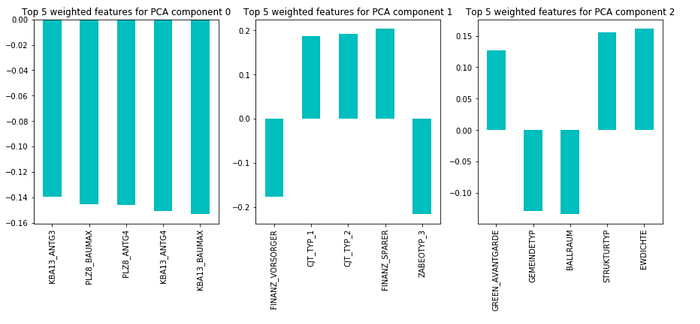
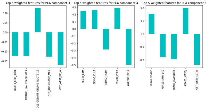
kmeans = KMeans(n_clusters=6, random_state=42, n_jobs=-1).fit(azdias_pca)The top 5 important PCA components for each cluster is shown below

Comparison between customers and the general population

I transformed the customers and the general population into 6 clusters separately, and the result is shown on the left.
general_clusters = kmeans.predict(azdias_pca)
customers_clusters  = kmeans.predict(customers_pca)
Cluster 4 has the highest positive difference in proportion between customers and the general audience. Clusters 1 and 5 have the highest negative difference in proportion between customers and the general audience. The composition of the major components for clusters 1,4,5 are shown below.
According to the above analysis, the client has a customer base advantage on those who care about environmental sustainability and with strong economic power; They are also interested in advertising over different channels.
Supervised Learning: Response Prediction
Now that I’ve found which parts of the population are more likely to be customers of the mail-order company, it’s time to build a prediction model. Each of the rows in the “MAILOUT” data files represents an individual that was targeted for a mailout campaign. I used the demographic information from each individual to decide whether or not it will be worth it to include that person in the campaign.
There is a large output class imbalance, where most individuals did not respond to the mailout. Thus, predicting individual classes and using accuracy does not seem to be an appropriate performance evaluation method. Instead, I used AUC to evaluate performance.
First, I tried four basic models: Logistic Regression, Random Forest Classifier, Gradient Boosting Classifier, and Support Vector Classification

The area under the ROC curve is the AUC score, and I found Gradient Boosting Classifier gives the best result: the AUC score for LR is 0.67; for RFC is 0.52; for GBC is 0.73; for SVC is 0.58. Then, I used GridSearchCV to tune the parameters in Gradient Boosting Classifier in order to improve performance.
parameters = {
 “learning_rate”: [0.1,0.2],
 “min_samples_split”: [2,5,8],
 “max_depth”:[3,5,8]}gbc = GradientBoostingClassifier(random_state=42)
cv = GridSearchCV(estimator = gbc, param_grid = parameters,scoring = “roc_auc”, cv =2,n_jobs = -1,verbose=3)
cv.fit(X_train,y_train)
It turned that the best parameters are {‘learning_rate’: 0.1, ‘max_depth’: 3, ‘min_samples_split’: 2}. The mean cross-validated AUC score of the best_estimator is 0.66, the validation data AUC score is 0.73.
Finally, I used this model to make predictions.
best_gbc=cv.best_estimator_test_cleaned_pre=test_cleaned.drop("LNR",axis=1)
pred_test=best_gbc.predict_proba(test_cleaned_pre)[:,1]
Kaggle Competition

I test that model in competition through Kaggle, and my model produced an AUC score of 0.78
