Customer analytics and response prediction for Arvato-part 1

• Capstone Project for Udacity Data Scientist NanoDegree

Image source: https://xaltius.tech/why-is-data-cleaning-important/

Introduction

This project aims to analyze how can a client of Bertelsmann Arvato acquires new customers more efficiently. The client is a mail-order company in Germany that sells organic products. Instead of reaching out to the general population, the client can reach out to people that identified as being the most likely to become new customers.

There are four major parts:

1. Data exploration and preprocessing
2. Customer segmentation: I analyzed demographics data for customers through unsupervised learning techniques, comparing it against demographics information for the general population, identified the parts of the population that best describe the company’s core customer base.
3. Response Prediction: I made a model to predict which individuals are most likely to convert into becoming customers for the company.

4. Kaggle Competition

Due to the length of the article, this post will focus on the first part of the project and part 2 will focus on parts 2,3, and 4.

Data exploration and preprocessing

There are five data files associated with this project:

• Udacity_AZDIAS_052018.csv: Demographics data for the general population of Germany; 891 211 persons (rows) x 366 features (columns).
• Udacity_CUSTOMERS_052018.csv: Demographics data for customers of a mail-order company; 191 652 persons (rows) x 369 features (columns).
• Udacity_MAILOUT_052018_TRAIN.csv: Demographics data for individuals who were targets of a marketing campaign; 42 982 persons (rows) x 367 (columns).
• Udacity_MAILOUT_052018_TEST.csv: Demographics data for individuals who were targets of a marketing campaign; 42 833 persons (rows) x 366 (columns).
• DIAS Attributes - Values 2017.xlsx: A detailed mapping of data values for each feature in alphabetical order.

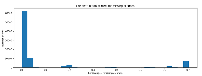
The first four datasets are basically the same in column names. As we can see in the following screenshot, there are a lot of missing values, so dealing with missing values is an important cleaning step in this project.

The head of the dataset

Deal with ‘unknown’s

Before dropping or imputing missing values, I took some efforts to make sure I found all the missing values. There are many columns that have a mapping for “unknown” values. These “unknown” need to be replaced with NaNs.

The head of mapping of data values for each feature

Remove unnecessary columns

Some columns are not unnecessary for this project since they are redundant or meaningless for analysis. I removed those columns for better interpretation and modeling building

1. Columns that convey duplicate information

• LP_FAMILIE_GROB and LP_FAMILIE_FEIN
• LP_STATUS_GROB and LP_STATUS_FEIN
• LP_LEBENSPHASE_GROB and LP_LEBENSPHASE_FEIN
• CAMEO_DEUG_2015 and CAMEO_DEU_2015

These pairs focus on the same attributes, but FEINs and DEU are more detailed. So I retained one from each pair. Usually, it is better to keep detailed information, but LP_LEBENSPHASE_FEIN has too many unique values. After considering all the factures together, LP_FAMILIE_GROB,LP_STATUS_GROB,LP_LEBENSPHASE_FEIN,CAMEO_DEUG_2015 could be dropped.

2. Columns meaningless for analysis

Some columns don't provide useful information for this project, so I removed them to make the dataset concise.

• LNR — an ID column
• EINGEFUEGT_AM — a date column with unknown meaning (not in the attributes file) and with too many unique values
• EINGEZOGENAM_HH_JAHR — a year column with unknown meaning (not in the attributes file)and with too many unique values
• D19_LETZTER_KAUF_BRANCHE — a feature name colum (not in the attributes file)
• MIN_GEBAEUDEJAHR — year the building was first mentioned in our database, irrelevant to the analysis

Remove columns and rows with too many with missing values

The missing value is a major problem in this dataset, and columns with more than 30% of data missing should be removed.

Features with more than 30% of missing data

Row with more than 50% of columns missing can be dropped.

The distribution of rows for missing columns

Imputing missing values

After dropping rows and columns with too many missing values, there are still a lot of missing ones. I used different approaches to impute missing values for different kinds of variables. A categorical variable is one that has two or more categories, but there is no intrinsic ordering to the categories. An ordinal variable is a categorical variable for which the possible values are ordered. I use mode to impute categorical variables, mean values to impute numerical variables, and median to impute ordinal variables.

for col in cat_cols:
    azdias[col].fillna(azdias[col].mode()[0], inplace=True)
for col in num_cols:    
    azdias[col].fillna((azdias[col].mean()), inplace=True)
for col in ord_cols:    
    azdias[col].fillna((azdias[col].median()), inplace=True)

Convert categorical variables into dummy variables

To make future analysis easier, I converted all the categorical variables into dummy variables. 21 categorical variables are turned into 124 dummy variables.

dummies_df = pd.get_dummies(azdias[cat_cols], drop_first=True)
azdias.drop(cat_cols, axis=1, inplace=True)

Remove outliers for numeric variables

Having outliers often has a significant effect on analysis. Because of this, I must take steps to remove outliers from our data sets.

Q1 and Q3 represent the first and third quantiles respectively, and IQR is the difference between Q3 and Q1. The lower limit for a column is Q1-1.5 IQR and the upper limit for a column = Q3 + 1.5 IQR
If the column has skewness more than 1 or less than -1, outlier treatment needs to be done: any values greater than the upper limit are replaced with the upper limit; any values lower than the lower limit are replaced with the lower limit.

for col in skewed_cols: 
    Q1 = df[col].quantile(0.25)
    Q3 = df[col].quantile(0.75)
    IQR = Q3 — Q1
    lower = Q1–1.5*IQR
    upper = Q3 + 1.5*IQR
    df[col] = np.where(df[col] <lower, lower, df[col])
    df[col] = np.where(df[col] >upper, upper, df[col])

Feature Scaling

Before I applied dimensionality reduction techniques and prediction models, I performed feature scaling so that the variables would not be influenced by the natural differences in scale for features. Since the numerical data is not Gaussian-like, I use normalization instead of Standardization.

norm = MinMaxScaler()
azdias_cleaned=norm.fit_transform(azdias)
azdias_cleaned=pd.DataFrame(azdias_cleaned,index=azdias.index, columns=azdias.columns)
azdias_cleaned.head(10)

Now the data preprocessing process is finished, in order to make the process easier for the remaining three datasets, I created a function that groups all the processes together. I can pass the dataset I want to clean and then get a cleaned dataset back.

In the next post, I will discuss the remaining three steps of the project.